Information Sheet and Assignment Number 8
Methods of Linear Correlation Objectives
Upon completion of this package, you will be able to:
- Explain the difference between statistical correlations and true causality.
- Evaluate different sets of data as to the appropriate type of correlation needed for analyzing the data.
- Compute Pearson Product Moment Correlations (r).
- Compute Spearman Rank Order Correlation (rho).
- Interpret the results of coefficients of correlation.
Reading Assignments
Urdan, pp. 79-92.
Lang and Heiss, pp. 30-31.
Materials presented in this package.
Turney & Robb, pp. 95-100.
Isaac & Michael, pp. 176, 177, 202, 204.
Tuckman, pp. 276-279, 288-289.
Evaluation
- Cite the difference between statistical correlations and true causality.
- When and why would you employ Pearson's r?
- When and why would you employ Spearman's rho?
- Compute Pearson's r for the following data:
| Subject
| X |
Y |
|
Subject |
X |
Y |
| S1 |
1 |
7 |
|
S5 |
9 |
10 |
| S2 |
3 |
4 |
|
S6 |
11 |
22 |
| S3 |
5 |
13 |
|
S7 |
13 |
19 |
| S4 |
7 |
16 |
|
|
|
|
- Compute Spearman's Rho for the following data:
| Q Rank |
Leadership Rank |
|
Q Rank |
Leaderhip Rank |
|
Q Rank |
Leadership Rank |
| 1 |
4 |
|
6 |
10 |
|
11 |
11 |
| 2 |
2 |
|
7 |
8 |
|
12 |
6 |
| 3 |
9 |
|
8 |
13 |
|
13 |
12 |
| 4 |
1 |
|
9 |
5 |
|
14 |
15 |
| 5 |
7 |
|
10 |
3 |
|
15 |
14 |
- Explain what the results of problems 4 and 5 indicate to you and their use in research.
- Problem 4 - Pearson's r
H1: Workers who score well on safety instruction will compare on a job satisfaction survey.
- Problem 5 - Spearman's Rho
H1: Students with high quality point averages while in college will display leadership qualities on the job.
METHODS OF RESEARCH IN EDUCATION
OTED 635
Information Sheet
Methods of Linear Correlation
LINEAR CORRELATION
When we speak of correlation, we are interested in the relation between two or more variables. One frequent assumption in psychology is that two variables have a linear relationship. This means that the relationship between the two variables can be portrayed as a straight line. This package will introduce you to two methods of linear correlation.
Coefficients of correlation measure the degree of relationship between variables in terms of the change in those variables. As the days get progressively colder, the number of insects left in the air becomes smaller and smaller. If we let the temperature on a given day be X, and the number of flying insects on a given day be Y, we can take measurements of both X and Y over a period of several days and see if there is any statistical relationship between these measurements.
The two types of correlations we are going to discuss are used for relating two variables, one X and one Y. Our data will consist of pairs of numbers, an X measurement and a Y measurement.
PEARSON'S r
The most commonly computed statistical coefficient of correlation is r. The basic requirement of this method of correlation is that both sets of measurements be at least interval data. We do not use Pearson's r with ordinal numbers.
COMPUTATION OF r
The Pearson product-moment correlation (r) is used to determine if there is a relationship between two sets of paired numbers. Generally, the paired numbers are (1) two different measures on each of several objects or persons, or (2) one measure on each of several pairs of objects or people where the pairing is based on some natural relationship, such as father to son, or on some initial matching recording to one specific variable, such as IQ score.
Assume that an experimenter wishes to determine whether there is a relationship between the grade point average (GPA's) and the scores on a reading-comprehension test of fifteen college freshman.
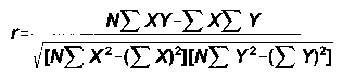
The basic computational formula for the Pearson product-moment correlation is:
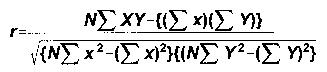
where: N = number of pairs of scores
XY = sum of the products of the paired scores
X = sum of scores on one variable
Y = sum of scores on the other variable
X2 = sum of the squared scores on the X variable
Y2 = sum of the squared scores on the Y variable
Step 1. The scores must be paired in some meaningful way in order to use the Pearson r. In the present example, the two different scores -- reading comprehension and grade point average -- are paired and recorded for each of the fifteen students:
| Student |
Reading
Score (X) |
Freshman
GPA (Y) |
|
Student |
Reading
Score (X) |
Freshman
GPA (Y) |
|
Student |
Reading
Score (X) |
Freshman
GPA (Y) |
| S1 |
38 |
2.1 |
|
S6 |
61 |
3.7 |
|
S11 |
48 |
3.4 |
| S2 |
54 |
2.9 |
|
S7 |
57 |
3.2 |
|
S12 |
46 |
2.5 |
| S3 |
43 |
3.0 |
|
S7 |
25 |
1.3 |
|
S13 |
44 |
3.4 |
| S4 |
45 |
2.3 |
|
S9 |
36 |
1.8 |
|
S14 |
39 |
2.6 |
| S5 |
50 |
2.6 |
|
S10 |
39 |
2.5 |
|
S15 |
48 |
3.3 |
Step 2. Multiply the two numbers in each pair; then add the products.
(38 x 2.1) + (54 x 2.9) +...+ (48 x 3.3) = 1889.4
Step 3. Multiply the number obtained in Step 2 by N, the number of paired scores (15 in this example).
1889.4 x 15 = 27341
Step 4. Square each number in the first column, and add the squared values.
382 +542 + ... + 482 = 31327
Step 5. Multiply the sum of Step 4 by the number of paired scores (N = 15 in this example).
31,327 x 15 = 469905
Step 6. Add all the scores in the first column (in this example, the reading-comprehension scores).
38 + 54 + ... + 48 = 673
Step 7. Square the value obtained in Step 6.
6732 = 452929
Step 8. Square each number in the second column, and add the squared values. (Note: The value of Step 10 can be obtained at the same time, as explained in Step 4.)
2.12 + 2.92 + ...3.32 = 116
Step 9. Multiply the result of Step 8 by the number of paired scores (N = 15 in this example).
110.2 x 15 = 1740
Step 10. Add all the scores in the second column (in this example, the freshman GPA's).
2.1 + 2.9 + ... + 3.3 = 40.6
Step 11. Square the value obtained in Step 10.
39.62 = 1648.36
Step 12. Multiply the final value of Step 6 by that of Step 10.
673 x 39.6 = 27323.8
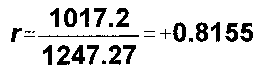
Step 13. The numerator of r is now computed by subtracting the value obtained in Step 12 from that obtained in Step 3.
28341 - 27323.8 = 1017.2
Step 14. Subtract the value of Step 7 from that of Step 5.
469905 - 452929 = 16976
Step 15. Subtract the final value of Step 11 from that of Step 9.
1740 - 1648.36 = 91.64
Step 16. Multiply the result of Step 14 by the result of Step 15.
16976 x 91.64 = 1555680.6
Step 17. Take the square root of the result of Step 16.
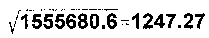
Step 18. Divide the value of Step 13 by that of Step 17. This yields the value of the Pearson product-moment correlation.
SPEARMAN's Rho
Spearman's Rho is a correlation coefficient built on the same structure as Pearson's r, only for use with ordinal data. It is very useful for correlating rankings and other ordinal data.
COMPUTATION OF Rho
Spearman's rho is used when an experimenter wishes to determine whether two sets of rank-ordered data are related.
The experimenter first asked an experienced teacher to rank twenty children in her class according to what she believed their intelligence to be. Then the children were tested and their actual Wechsler IQ scores obtained. The data were as follows:
| Child |
Teacher's
Ranking |
IQ Score |
|
Child |
Teacher's
Ranking |
IQ Score |
| A |
1 |
116 |
|
K |
11 |
116 |
| B |
2 |
111 |
|
L |
12 |
109 |
| C |
3 |
97 |
|
M |
13 |
103 |
| D |
4 |
122 |
|
N |
14 |
103 |
| E |
5 |
116 |
|
O |
15 |
96 |
| F |
6 |
105 |
|
P |
16 |
90 |
| G |
7 |
108 |
|
Q |
17 |
134 |
| H |
8 |
95 |
|
R |
18 |
87 |
| I |
9 |
124 |
|
S |
19 |
96 |
| J |
10 |
98 |
|
T |
20 |
91 |
The following formula for rho (p) describes the computational procedure.
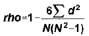
Where d = difference of score between each X and Y pair
N = number of pairs of scores
Step 1. Rank the IQ scores so that both variables are ranked.
Note: When two children have the same IQ score, the same rank is given to each. But notice that the rank given is the mean value of the two ranks for the two tied scores. For example, Child M and Child N both have IQ scores of 103. These scores should fall into ranks 11 and 12, but since both children have the same IQ score, both are ranked as 11.5 and the next score (Child J. with and IQ score of 98) is ranked as 13.
| Child |
Teacher's
Ranking |
IQ Score |
IQ Rank on
the basis of
test score |
|
Child |
Teacher's
Ranking |
IQ Score |
IQ Rank on
the basis of
test score |
| A |
1 |
116 |
5 |
|
K |
11 |
116 |
5 |
| B |
2 |
111 |
7 |
|
K |
11 |
116 |
5 |
| C |
3 |
97 |
14 |
|
M |
13 |
103 |
11.5 |
| D |
4 |
122 |
3 |
|
N |
14 |
103 |
11.5 |
| E |
5 |
116 |
5 |
|
O |
15 |
96 |
15.5 |
| F |
6 |
105 |
10 |
|
P |
16 |
90 |
19 |
| G |
7 |
108 |
9 |
|
Q |
17 |
134 |
1 |
| H |
8 |
95 |
17 |
|
R |
18 |
87 |
20 |
| I |
9 |
124 |
2 |
|
S |
19 |
96 |
15.5 |
| J |
10 |
98 |
13 |
|
T |
20 |
91 |
18 |
Step 2. Compute the difference between the two ranks for each child. The resulting value is called the d value. List these values in a column, making sure to note whether they are positive or negative.
| Child |
d value |
|
Child |
d value |
|
Child |
d value |
|
Child |
d value |
| A |
-4 (1-5) |
|
F |
-4 (6-10) |
|
K |
+6 (11-5) |
|
P |
-3 (16-19) |
| B |
-5 (1-5) |
|
G |
-4 (6-10) |
|
L |
+6 (11-5) |
|
Q |
-3 (16-19) |
| C |
-11 (3-14) |
|
H |
-9 (8-17) |
|
M |
+1.5 (13-11.5) |
|
R |
-2 (18-20) |
| D |
+1 (4-3) |
|
I |
+7 (9-2) |
|
N |
+2.5 (14-11.5) |
|
S |
+3.5 (19-15.5) |
| E |
0 (5-5) |
|
J |
-3 (10-13) |
|
O |
-0.5 (15-15.5) |
|
T |
+2 (20-18) |
Step 3. Square all the d Values from Step 2, and add all the squared values.
(-42) + (-52) + . . . +22 = 668
Step 4. Multiply the result of step 3 by the number 6. (Note: The number 6 is always used, regardless of the number of ranks, etc., involved).
668 x 6 = 4008
Step 5. Compute N(N2-1). (In our example N = 20).
20(202 - 1) = 20(400 - 1) = 20(399) = 7980
Step 6. Divide the result of Step 4 by the result of Step 5.
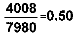
Step 7. Subtract the final value of Step 6 from the number 1. (Note: The number 1 is also always used.) This yields the value of Spearman's rho. Be careful to record whether it is positive or negative.
rho = 1 - 0.50 = + 0.50
Here is an example of a direct relationship:
| X |
Y |
|
| 2 |
15 |
|
| 4 |
20 |
|
| 6 |
25 |
r = +1.00 |
| 8 |
30 |
|
| 10 |
35 |
|
Once again we have a perfect set of data, but you can easily see the relationship. As one variable increases, the other also increases, or as one variable decreases, the other also decreases. This is what we call a direct relationship.
A FURTHER NOTE ON MAGNITUDE
It is difficult to say how large a correlation coefficient should be to be "meaningful". The strength of the relationship represented must be interpreted in the context of that relationship. In general, however, the student can follow this interpretation:
| CORRELATION VALUE |
APPROXIMATE MEANING |
| less than 0.20 |
Slight, almost neglible relationship |
| 0.20 to 0.40 |
Low correlation; definite bur small relationship |
| 0.40 to 0.70 |
Moderate correlation; substantial relationship |
| 0.70 to 0.90 |
High correlation; very dependable relationship |
| 0.90 to 1.00 |
Very high correlation; very dependable relationship |
CAUSALITY
It is important for the student to realize at this time that when we figure correlation, we are figuring the statistical degree of relationship between variables. We are not, much as you might think, determining whether one variable causes or influences the other. A very common mistake in social science is to interpret a high correlation as meaning causality. Thus, if A and B are highly correlated it does not necessarily follow that A causes B or B causes A. A common explanation would be that a third variable, C, causes both A and B thus making it look like they are related. Correlation is extremely useful for finding relationships and predicting trends, but is only the first step in trying to determine causality.
INTERPRETATION OF rho AND r
Correlation coefficients give us two pieces of information concerning the relationship between two variables; the strength of that relationship and its direction.
If computed correctly, the value of the correlation coefficient will always fall between -1 and +1. This is true for both rho and r. The strength of the relationship is shown by how large the coefficient is, that is, how close it is to plus or minus one. Here are some examples of "weak" coefficients:
Note that all of these coefficients are close to zero. This means that there is little statistical relationship between the two variables. Here are some examples of "strong" coefficients:
Note that all of these coefficients are close to one (positive or negative). Thus, we see that the size of the number (between zero and one) is an indication of the strength of the relationship. The sign of the coefficient has nothing to do with strength. The sign of the coefficient merely reflects whether the relationship is direct (positive sign) or indirect (negative sign).
Here is an example of an indirect relationship:
| X |
Y |
|
| 5 |
1 |
|
| 4 |
2 |
|
| 3 |
3 |
r = -1.00 |
| 2 |
4 |
|
| 1 |
5 |
|
Of course, not all sets of data are this obvious, we very seldom get a perfect relationship between groups of data. The important thing to notice is that as one variable gets larger, the other gets smaller. This is what we mean by an indirect relationship.
Critical Values of the Pearson Product Moment Correlation Coefficient
| |
Level of significance for one-tailed test |
df = N - 2
(degrees of
freedom) |
0.05 |
0.025 |
0.01 |
0.005 |
0.0005 |
| Level of significance for two-tailed test |
| 0.10 |
0.05 |
0.02 |
0.01 |
0.001 |
| 1 |
.9877 |
.9969 |
.9995 |
.9999 |
1.0000 |
| 2 |
.9000 |
.9500 |
.9800 |
.9900 |
.9990 |
| 3 |
.8054 |
.8783 |
.9343 |
.9587 |
.9912 |
| 4 |
.7293 |
.8114 |
.8822 |
.9172 |
.9741 |
| 5 |
.6694 |
.7545 |
.8329 |
.8745 |
.9507 |
| 6 |
.6215 |
.7067 |
.7887 |
.8343 |
.9249 |
| 7 |
.5822 |
.6664 |
.7498 |
.7977 |
.8982 |
| 8 |
.5494 |
.6319 |
.7155 |
.7646 |
.8721 |
| 9 |
.5214 |
.6021 |
.6851 |
.7348 |
.8471 |
| 10 |
.4973 |
.5760 |
.6581 |
.7079 |
.8233 |
| 11 |
.4762 |
.5529 |
.6339 |
.6835 |
.8010 |
| 12 |
.4575 |
.5324 |
.6120 |
.6614 |
.7800 |
| 13 |
.4409 |
.5139 |
.5923 |
.6411 |
.7603 |
| 14 |
.4259 |
.4973 |
.5742 |
.6226 |
.7420 |
| 15 |
.4124 |
.4821 |
.5577 |
.6055 |
.7246 |
| 16 |
.4000 |
.4683 |
.5425 |
.5897 |
.7084 |
| 17 |
.3887 |
.4555 |
.5285 |
.5751 |
.6932 |
| 18 |
.3783 |
.4438 |
.5155 |
.5614 |
.6787 |
| 19 |
.3687 |
.4329 |
.5034 |
.5487 |
.6652 |
| 20 |
.3598 |
.4227 |
.4921 |
.5368 |
.6524 |
| 25 |
.3233 |
.3809 |
.4451 |
.4869 |
.5974 |
| 30 |
.2960 |
.3494 |
.4093 |
.4487 |
.5541 |
| 35 |
.2746 |
.3246 |
.3810 |
.4182 |
.5189 |
| 40 |
.2573 |
.3044 |
.3578 |
.3932 |
.4896 |
| 45 |
.2428 |
.2875 |
.3384 |
.3721 |
.4648 |
| 50 |
.2306 |
.2732 |
.3218 |
.3541 |
.4422 |
| 60 |
.2108 |
.2500 |
.2948 |
.3248 |
.4078 |
| 70 |
.1954 |
.2319 |
.2737 |
.3017 |
.3799 |
| 80 |
.1829 |
.2172 |
.2565 |
.2830 |
.3568 |
| 90 |
.1729 |
.2050 |
.2422 |
.2673 |
.3375 |
| 100 |
.1638 |
.1946 |
.2301 |
.2540 |
.3211 |
Table VI - Critical Values of rs, the Spearman Rank Correlation Coefficient
| N |
Significance level (one-tailed test) |
| 4 |
1.000 |
|
| 5 |
.900 |
1.000 |
| 6 |
.829 |
.943 |
| 7 |
.714 |
.893 |
| 8 |
.643 |
.833 |
| 9 |
.600 |
.783 |
| 10 |
.564 |
.746 |
| 12 |
.506 |
.712 |
| 14 |
.456 |
.645 |
| 16 |
.425 |
.601 |
| 18 |
.399 |
.564 |
| 20 |
.377 |
.534 |
| 22 |
.359 |
.508 |
| 24 |
.343 |
.485 |
| 26 |
.329 |
.465 |
| 28 |
.317 |
.448 |
| 30 |
.306 |
.432 |
CORRELATION
Some problems in educational or psychological research necessitate the comparison of two sets of measures, such as test scores, in order to determine whether the measures show a relationship. That is, it is necessary to find out if there is a correlation between the variables. If the variables are found to rise or fall together in such a way that an increase in one is accompanied by an increase in the other or a decrease in one is accompanied by a decrease in the other, there is a positive correlation. The correlation is negative or inverse if an increase in one variable is accompanied by a decrease in the other. An example of a positive correlation is found in a comparison of height and weight. Generally speaking, taller people tend to be heavier than shorter people. An example of a negative relationship is the correlation between horsepower and gas mileage in automobiles: generally speaking, as horsepower increases, mileage decreases.
Karl Pearson, a mathematician of great renown, developed a statistical procedure for obtaining a coefficient of correlation that is commonly employed today when a numerical value is needed to express the degree of relationship between variables. The symbol for a Person product-moment coefficient of correlation is r. When r is zero, no correlation exists between two variables, such as X and Y. When r is +1.00, there is a perfect positive correlation, and when it is -1.00, there is perfect negative correlation. We shall discuss the interpretation of a correlation coefficient a little later in this chapter.
The use of a scatter diagram or scattergram will permit the researcher to show graphically the relationship between two sets of measures, such as scores from Test X and Test Y. The scattergram also will reveal whether the relationship between the scores is linear (straight line) or nonlinear. The Person r applies only to the linear relationships. A scattergram for the following sets of data appears in Figure 1.
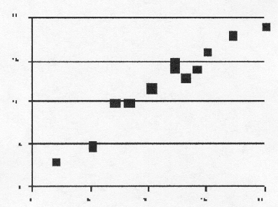
Figure 1. A scattergram for scores on Test X and Test Y.
| Student Number |
Score on Test X |
Score on Test Y |
| 01 |
20 |
19 |
| 02 |
17 |
18 |
| 03 |
15 |
16 |
| 04 |
14 |
14 |
| 05 |
13 |
13 |
| 06 |
12 |
15 |
| 07 |
12 |
14 |
| 08 |
10 |
12 |
| 09 |
8 |
10 |
| 10 |
7 |
10 |
| 11 |
5 |
5 |
| 12 |
2 |
3 |
In the scattergram a point has been positioned on the graph to show the corresponding values of X and Y for each of the 12 students. For example, student number 01 has a score of 20 for Test X and a score of 19 for Test Y. A single point was made on the graph to show where the two values intersect. It can be seen that the pattern of points is linear and could be represented by a line running from the lower left of the graph to the upper right. This tells us that the relationship is linear and positive. Had the pattern run from the upper left to the lower right the correlation would have been negative. Three examples of scattergrams for positive, negative, and zero correlation are shown in Figure 2.
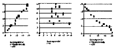
Figure 2. Examples of scattergrams.
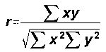
PRODUCT-MOMENT COEFFICIENT OF CORRELATION
The basic formula for finding the Pearson r is written
where
x = X-
y = Y-
N = The number of pairs of scores

xy = The sum of the products of the deviations from the means of X and Y respectively
A variation of the basic formula is the following:
Since the use of calculators and computers is becoming more and more widespread, the following raw-score formula is especially useful for computing r.
We shall use the raw-score formula to demonstrate the calculation of a coefficient of correlation for the scores made by students selected at random from a larger group (population).
ENGLISH AND SOCIAL STUDIES ACHIEVEMENT TEST SCORES FOR TWELVE STUDENTS
| ENGLISH TEST SCORES (X) |
SOCIAL STUDIES TEXT SCORES (Y) |
| 40 |
38 |
| 36 |
36 |
| 32 |
40 |
| 30 |
35 |
| 28 |
30 |
| 25 |
20 |
| 25 |
32 |
| 25 |
28 |
| 22 |
25 |
| 20 |
22 |
| 20 |
20 |
| 15 |
18 |
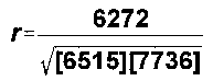
In order to compute r for the preceding data, we will need the following values:
- The number of pairs of scores, or N.
- The sum of the products of the pairs of scores, or XY
- The sum of the scores for Test X.
- The sum of the scores for Test Y.
- The sum of the squared scores for Test X.
- The sum of the squared scores for Test Y.
| X |
X2 |
Y |
Y2 |
XY |
| 40 |
1600 |
38 |
1444 |
1520 |
| 35 |
1225 |
36 |
1296 |
1260 |
| 32 |
1024 |
40 |
1600 |
1280 |
| 30 |
900 |
35 |
1225 |
1050 |
| 28 |
784 |
30 |
900 |
840 |
| 25 |
625 |
20 |
400 |
500 |
| 25 |
625 |
32 |
1024 |
800 |
| 25 |
625 |
28 |
784 |
700 |
| 22 |
484 |
25 |
625 |
550 |
| 20 |
400 |
22 |
484 |
440 |
| 20 |
400 |
20 |
400 |
400 |
| 15 |
225 |
18 |
324 |
270 |
 X=317 X=317 |
=8917 |
Y=344 |
Y2=10,560 |
XY=9610 |
INTERPRETATION OF A CORRELATION COEFFICIENT
How should be interpret the r of .88 just computed?
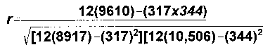
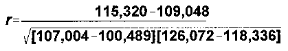
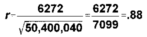
First of all we must determine whether it is statistically significant. A formula can be used for the purpose, but it is simpler to use a table, such as Table D in the Appendix. In Table D the first column shows degrees of freedom (df). In the previous problem, df=10, because we find df by the formula N-2, where N equals the number of pairs of scores. After locating 10 in the df column, we can find the figure .576 in the 5 percent column and .708 in the 1 percent column. Our computed r of .88 exceeds both these values, so it is significant at the 1 percent level. We can conclude that this r represents an estimate of a population coefficient of correlation between the variables X and Y that is greater than zero.
Since we have accepted the coefficient of correlation as statistically significant, we can proceed with our interpretation. The interpretation of r must take into account two things: the sign of r and the size of it. The sign (positive or negative) tells us about the direction of the relationship. Our computed r of .88 is positive, so we know that the correlation is positive. It is relatively difficult, however, to interpret the size of a correlation coefficient. It should be emphasized that r's are not to be interpreted as are percents. Our r of .88 definitely does not imply that X and Y are correlated 88 percent of the time. Furthermore, we cannot say that an r of .88 shows twice as strong a relationship between two variables as an r of .44. Actually, .88 shows more than twice the relationship that .44 shows. If we square an r we can determine the amount of variation in a second variable that is associated with variation in the first. For example, if we square an r of .88 we get .77. Now we can say that 77 percent of the variation in out Test X scores is associated with the variation in Test Y scores, or vice versa.
As a rough guide to providing qualitative descriptive terms for coefficients of correlation, the following system is suggested:
| CORRELATION VALUE |
APPROXIMATE MEANING |
| less than 0.20 |
Slight, almost neglible relationship |
| 0.20 to 0.40 |
Low correlation; definite bur small relationship |
| 0.40 to 0.70 |
Moderate correlation; substantial relationship |
| 0.70 to 0.90 |
High correlation; very dependable relationship |
| 0.90 to 1.00 |
Very high correlation; very dependable relationship |
It should be emphasized that correlation does not necessarily imply causation. Or, in other words, even if a very high and statistically significant correlation coefficient is obtained the assumption should not be made that X causes Y or that variables are affected by another variable or variables and do not affect each other directly.