METHODS OF RESEARCH IN EDUCATION OTED 635 Types of Data Due to the differences in the way in which we measure things, the numbers we accumulate do not always mean the same thing. We still divide the numbers which researchers commonly encounter into three scales of data. Almost all numbers fall into one of these three data types. INTERVAL Interval numbers are those numbers with which you are probably most familiar. As you can see from the number line, interval numbers are called so because the intervals between the numbers are equal. Some people call this type of data equidistant interval data. However, we simply call it interval data. Interval data is probably the most common type of data which we run into in educational research, the reason for this being that most standardized or classroom tests give us scores which can be interpreted as being interval in nature. For instance, if John gets a 20 on a test and Frank gets a 25 we assume the difference in these two scores to represent 5 units of knowledge or ability. Since these numbers do have equal intervals between them we can perform the usual arithmetic operations such as addition, subtraction, multiplication, and division. For this reason we can figure the mean with interval data. This is very important because being able to figure the mean is a first step in the use of most higher level statistical analyses. ORDINAL Ordinal data are commonly encountered by researchers, but not as commonly as interval data. The most distinguishing characteristic of ordinal data is the fact that when placed on the line, the numbers do not have equal intervals between them. As you can see, although the numbers do get larger as we go to the right, we don't know how much larger they get.
Most ordinal data which is encountered by researchers comes to us in the form of ordinal ranks. Whenever we ask people to rank objects or attributes or other people in order of preference or in order on some scale, we are generating ordinal data. This is very important to remember. NOMINAL Nominal numbers themselves are seldom encountered in educational research. An example of a nominal number for instance, would be the numbers on a football jersey. The numbers mean nothing in terms of actual quantifications. They do, however, serve to label. For this reason we call them nominal numbers. Nominal data are usually encountered by researchers when we categorize things. For instance, we may count the number of apples, pears, peaches, and oranges produced by a certain farmer. Whenever we count things and then place them into categories, we are developing nominal data from a research point of view. One of the most common forms of nominal data which we encounter in research are the results of questionnaire studies. When we count the number of people who respond to Item A, Item B, Item C, etc. MEASURES OF CENTRAL TENDENCY The behavior of an individual on a particular occasion may, or may not be typical of him. Therefore, it is often necessary to measure his behavior several times in order to get a good estimate of what he is likely to do. For example, suppose a man is being considered for an assignment as an astronaut. It is necessary to make certain he can react quickly to signals from the instruments in his space capsule. To test this, he is asked to press a button when a visual or an auditory signal is presented. His reaction time - the time required to press the button after the presentation of the stimulus - is then measured. THE MEAN To illustrate the problem of obtaining a measure of central tendency, consider an experiment in which a subject moved a control knob whenever he heard a signal. The time between the presentation of the signal and the movement of the knob was measured for twenty trials. The times are given in the Table. INDIVIDUAL REACTION TIMES
Although there is quite a range of measurements for this subject, the times seem to cluster around 160 milliseconds. Some times are several milliseconds away from this value, but half are within 10 milliseconds of 160. This clustering of measurements would be more apparent if the raw data were arranged in a frequency distribution. COMPUTING THE MEAN To express in mathematical terms the method of finding the mean, let the letter X stand for the score on each trial. Thus X1 could stand for the time of the first trial, X2 the time on the second trial, X5 the time on the fifth trial, and so on to Xn the nth or last score obtained. The arithmetic mean is designated by
This formula says that, regardless of how many observations are made, the mean is always equal to the sum of the values for all of the observations, divided by the number of observations. The formula presented above is inconveniently long to write, so it is usually given in a briefer form in which the instruction to add together all of the X's is indicated by the symbol for summation,
One must always remember that
What has been said about finding the mean reaction time of one subject can also be said about finding the mean reaction time of a group of individuals. In the latter case, the mean for each individual is represented by X value. Thus, the mean time for the first subject (S1) is represented by X1, the mean for S2 by X2, and the mean for the nth subject Xn. Suppose the mean reaction times of twelve subjects have been obtained by the method used in the earlier example. The means are shown in the Table: Mean Reaction Times for Twelve Subjects
Here, the
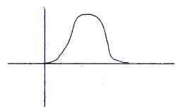
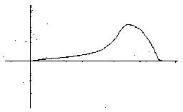
N = 12 That is, the mean score of a group of individuals is obtained by dividing the sum of their scores by the number of individuals in the group. THE MEDIAN A second measure of central tendency is the median. The median is the value above which half of the measure lie. It is used when the distribution is badly skewed -- when the measures are piled up at one end of the distribution rather than being more or less symmetrically distributed about the mean. The difference between symmetrical and skewed distributions can be seen below. When a distribution is skewed, the median is a better indicator of the central point about which most of the scored cluster.
Symmetrical and Skewed distributions The achievement test scores from a class of thirty students, some of whom had been promoted without being prepared, appear below: Achievement Test Scores
The mean of this distribution is 58, but two-thirds of the students did better than this. The median is 63, since half of the scores are above this value. In this example the median is more indicative of typical performance of the unprepared students. THE MODE A third measure of central tendency is the mode. The mode is the score that most frequently occurs. In the distribution of achievement test scores given above, the mode is 67 because more subjects had this score than any other. The mode is seldom used in statistics, but it is a quickly found measure of central tendency, since it can be easily identified without computation. In those cases where it typically is required, the mode provides the necessary information. The following table lists the number of errors made by twenty rats that learned a maze. Errors in Learning a Maze
The two modes of this distribution are at 8 and 13. SUMMARY We have then, three different measures of central tendency. Each measure is used for different purposes, and has different limitations as to use. MEAN The mean is best used to describe the average of a distribution of numbers that is fairly symmetrical. That is, a distribution without extreme scores at one end. Because it is used so much in statistics, the mean is the most important measure of central tendency for statisticians. One limitation is that the mean must be figured from interval or ratio data. We cannot take the mean of ordinal numbers, since we don't know how far the numbers are from each other in terms of distance. Most experiments involve comparing mean behavior, or mean performance between different groups. MEDIAN The median is best used to describe the middle of a distribution of numbers which has extreme values at one end or the other. Remember that the median is not affected by extreme scores as is the mean. A very common use of the median is to evaluate the central tendency of ordinal data (such as ranks), since we cannot compute the mean of such data. MODE The mode is seldom used in statistics. If it is used, the mode is usually found for one of these reasons:
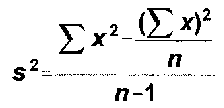
MEASURES OF VARIABILITY The mean, or some other measure of central tendency, is useful in determining what is representative behavior for an individual or group. It does not provide answers to such questions as, "How well does the measure of central tendency represent the group?" To answer these questions it is necessary to consider how the values in a distribution vary from one another and from the mean. This "spread" or dispersion in a set of measurements is called variability. Range The simplest measure of variability is the range. The range is the difference between the two extreme values in the distribution. Consider a distribution of scores (representing trials to an errorless performance) made by a group of girls on a finger maze: 3, 5, 6, 8, 9, 11, 12, 18, and 14. The range is equal to the highest value minus the lowest value: 14 - 3 = a range of 11. VARIANCE A measure of variability will describe a group of measurements better if it is based on every measurement in the group. It is also useful to give special weight or importance to those measurements that are the most unusual -- that is, those measurements farthest from the mean of the distribution. These conditions for a method of describing variation have been met in a statistic called the variance. The variance is defined as the mean of the squares of the deviations of each measurement from the mean. The formula for the variance (s2) is :
where
The variance includes all the data, because every measure in the group is used in its computation. Special weight is given to the extreme values because the deviation of each score is squared. The variance is a kind of average which reflects the distance of the individual scores from the mean of the distribution. The larger the variance, the greater the variability; that is, the greater the distance of scores from the mean. The smaller the variance, the less the variability. COMPUTING VARIANCE EXAMPLE This example is drawn from the area of development psychology. Assume that an experimenter is interested in obtaining information about the heights of twelve-year-olds. To do this, he collects a sample of data (the heights of twenty randomly selected twelve-year-olds) and proceeds to compute the variance. Step l. Table the data as follows. No particular order is necessary.
Step 2. Add all the scores. (Note: If you are using a calculator you can do Step 2 and Step 3 at the same time.) 64 + 48 + ... + 60=1208 Step 3. Square all the scores and add the squared values. 642 + 482 + ... + 602= 73,894 Step 4. Square the sum obtained in Step 2, and divide this value by the number of scores that were added to obtain the sum. The resultant value is called the correction term. Step 5. Subtract the value obtained in Step 4 from the sum in Step 3. 73,894 - 72,963 = 931 Step 6. Divide the value obtained in Step 5 by N - l.1 (In this example, it would be 20 - 1 = 19). The resultant value is the variance.
STANDARD DEVIATION The most commonly used measure of dispersion of a group of scores is not the range, nor the variance, but another statistic called the standard deviation. The standard deviation of a group of scores is an index of the degree to which the scores do or don't cluster around the mean. If we have a loose distribution with most scores right around the mean. The standard deviation is used quite often in statistics because it has certain mathematical properties which are quite useful in describing a group of scores. COMPUTATION Computation of the standard deviation from a distribution of numbers is quite simple. In fact, if you know how to find the variance, you are almost done finding the standard deviation. The reason for this is that the standard deviation equals the square root of the variance.
Therefore, to find the standard deviation of a group of scores, find the variance and take its square root. To find the standard deviation of our previous example, we would take the square root of the variance, which was 49, giving us a standard deviation of 7.
|
||||||||||||||||||||||||||||||||||||||||||||||||||||||||||||||||||||||||||||||||||||||||||||||||||||||||||||||||||||||||||||||||||||||||||||||||||||||||||||||||||||||||||||||||||||||||||||||||||||||||||||||||||||||||||||||||||||||||||||||||||||||||||||||||||||||||||||||||||||||||||||||||||||||||||||||||||||||||||||||||||||||||||||||||||||||||||||||||
|
|
||||||||||||||||||||||||||||||||||||||||||||||||||||||||||||||||||||||||||||||||||||||||||||||||||||||||||||||||||||||||||||||||||||||||||||||||||||||||||||||||||||||||||||||||||||||||||||||||||||||||||||||||||||||||||||||||||||||||||||||||||||||||||||||||||||||||||||||||||||||||||||||||||||||||||||||||||||||||||||||||||||||||||||||||||||||||||||||||

 (read " bar X") and the formula for finding the mean is:
 . The formula then becomes:
 or 159 milliseconds


 2
2

